Overview
Abstract
This BioGears Tissue system manages the extravascular space. It handles substance transport between the organs and the blood vessels, and it computes substance storage, transformation (e.g. chemical conversion), clearance, and excretion.
Introduction
The BioGears Tissue system is a low-resolution, mid-fidelity model of the tissues of the body. The system is mechanically tied to the Cardiovascular and Respiratory systems, and it interacts with the Energy and Drugs systems. The tissue system handles the non-advective transport of substances between the intravascular and extravascular spaces, as well as the conversion of substance (including chemical conversion of species and clearance/excretion). The metabolic production and consumption of substances takes place in the tissue system, and the tissues generate substances that are produced in the organs by any process or mode.
System Design
Background and Scope
Groups of cells in the body that share a common embryonic origin can be described collectively as a tissue. In the classical organizational hierarchy of organisms, tissues are at the level directly below organs, meaning that groups of tissues interacting to perform a function are an organ. There are four types of tissue in the human body: epithelial, connective, muscle, and nervous tissue. In BioGears, the term tissue refers to the extravascular space of an organ. In other words, in BioGears 'tissue' is a collective term that generally refers to the parenchyma.
Data Flow
Like the other BioGears systems, the Tissue system uses the execution structure described in System Methodology. Figure 1 shows the data flow.

Preprocess
At this time the there are no PreProcess steps in the Tissue System.
Process
Calculate Metabolic Consumption and Production
Conversions of nutrients to metabolic energy and byproducts are calculated for each relevant compartment.
Calculate Pulmonary Capillary Substance Transport
Gases are transferred from the lungs (alveoli) to the pulmonary capillaries and vice versa during this calculation. This allows for the transport of oxygen into the cardiovascular system from the ambient air, providing the required substances for metabolism. By the same process, carbon dioxide waste is removed from the Cardiovascular System and moves through the Respiratory System into the ambient air.
Calculate Diffusion
Substances move from the vascular space into and out of the extravascular or tissue space for metabolism, waste removal, and/ or clearance. This functionality moves gases across the membrane between the vascular and extravascular spaces using one or more of several diffusion models, discussed below.
- Perfusion Limited Diffusion
- Instant Diffusion
- Simple Diffusion
- Facilitated Diffusion
- Active Transport (Currently for sodium, potassium, and chloride)
Calculate Vital Signs
In this method the tissue volumes are summed in order to compute total body water. Body system level data is also set in this method. In the future, this method will compute and set tissue substance concentrations and trigger concentration-based events.
Protein Storage and Release
In this method, amino acid is stored or released from storage in muscle as dictated by the local hormone factor.
Fat Storage and Release
In this method, triacylglycerol is stored or released from storage in fat as dictated by the local hormone factor.
Post Process
At this time the there are no PostProcess steps in the Tissue System.
Assessments
Assessments in BioGears are data collected and packaged to resemble a report or analysis that might be ordered by a physician. No BioGears assessments are associated with the Tissue system.
Features, Capabilities, and Dependencies
The BioGears Tissue system is a low-resolution, mid-fidelity model of the tissues of the body. One of the primary functions of the BioGears Tissue system is to control the transport of substances between the tissues and the blood. There are several transport models that help the Tissue system perform that function. Figure 2 provides an overview of the extravascular space and the various modes of substance transport between the blood and the tissues. The BioGears Tissue system also handles the conversion of substance (i.e. metabolic consumption and production).
Bulk Flow and Advection
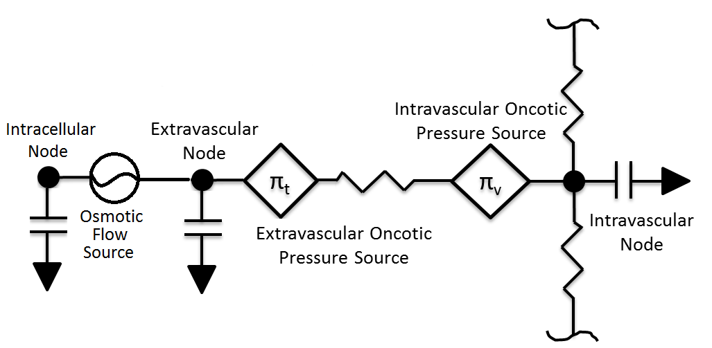
The movement of fluid between the intravascular and extravascular space is modeled using the BioGears Circuit Methodology. In most cases, each tissue circuit node is connected to one and only one cardiovascular circuit node. However, the gut tissue compartment is a lumped representation of the abdominal viscera organ tissues, and thus the large intestine, small intestine, and splanchnic vascular circuit nodes all connect to the gut tissue circuit node. Each tissue sub-circuit, a representative sample of which is shown in Figure 3, is modeled after the Starling Equation (Equation 1 below).
\[{J_v} = {K_f}\left( {\left[ {{P_c} - {P_t}} \right] - \sigma \left[ {{\pi _c} - {\pi _t}} \right]} \right)\]
Pc and Pt are the hydrostatic pressures stored on the vascular capillary and extracellular tissue nodes. The parameters KF and σ are the filtration and reflection coefficients, respectively. The filtration coefficient defines the tendency of fluid to pass into the extravasculature, and its inverse has units of resistance (hence the resistor element in Figure 3). The resistance of each tissue is assumed to be proportionate to its mass. The reflection coefficient describes the effectiveness of a membrane in maintaining an osmotic gradient on a 0 to 1 scalse. Finally, πc and πt capture the oncotic pressures generated by proteins in the plasma and interstitial fluids. As in the Renal Methodology, we assume that total plasma protein concentration is directly correlated with albumin concentration and use the Landis-Pappenheimer Equation to determine oncotic pressures. The current implementation assumes that all plasma proteins (including albumin) are too large to diffuse from the vascular space (that is, σ = 1) [gyenge1999transport], meaning that πc and πt maintain constant values. This decision is due to albumin leak to the interstitium generally being small and the lack of a BioGears lymph system to return albumin to the bloodstream. Under regular physiological conditions, this assumption is not unreasonable. However, in situations of rapid plasma osmolarity changes (as in during fluid administration), this assumption breaks down. To account for these situations, we calculate the mean concentrations of albumin in the vasculature and interstitial spaces. We then evaluate the Landis-Pappenheimer Equation in both the vasculature and intersitium using these mean concentrations and adjust the appropriate oncotic pressure source paths. This approach still neglects the possibility of albumin leak, which can occur in the leadup to hypovolemic shock. Future work will address the need for an accurate albumin diffusion model.
The volume in the tissue compartment is partitioned into the extracellular and intracellular space, as shown in Figure 2 and Figure 3. Fluid exchange between the extracellular and intracellular compartments of each tissue is directly calculated and set using a flow source. This process of intracellular volume regulation is inextricably linked with maintanance of ionic gradients; thus discussion of it is deferred to the Active Transport section. All substance transport into the tissue fluid space is simulated using one or more of the transport modes described below.
Patient Variability
The BioGears Tissue system is heavily dependent on the patient configuration. Fluid volume distributions and parenchyma masses both depend heavily on the patient sex, height, weight, and body fat fraction. Transport properties are also affected by patient variability. For example, permeability coefficients are computed from membrane permeability and membrane surface area, where the surface area is a function of the tissue mass, which in turn is a function of the patient weight. A detailed discussion of patient configuration and variability in BioGears is available in the Patient Methodology report.
Transport Processes
Perfusion-Limited Diffusion
Perfusion-limited diffusion is a technique for describing drug kinetics in physiology-based pharmacokintic models. Partition coefficents are using to compute the amount of a drug crossing a membrane at a given perfusion rate. The partition coefficients are calculated based on the physical chemical properties of the drug, the tissue properties of the organ, and the blood properties. They represent a specific substance’s affinity for moving across the blood-tissue partition. BioGears uses this methodology to simulate drug diffusion, and details of the partition coefficient calculation can be found in the Drugs Methodology. All current drugs in the BioGears Engine use perfusion-limited diffusion as found in [160] [149]. In the future, permeability-limited diffusion could be used. Equation 2 shows the calculation used to move mass from the vascular to the tissue and vice versa for perfusion-limited diffusion [160] .
\[\Delta M = Q_{T} * C_{V} - \frac{Q_{T} * C_{T}}{K_{P}} \]
Where ΔM is the change in mass due to diffusion, QT is the blood flow to the organ, CV is the concentration of the drug in the organ vasculature, CT is the concentration of the drug in the organ tissue, and KP is the partition coefficient for the drug and organ. This calculation is performed for each drug or substance and each tissue organ/compartment.
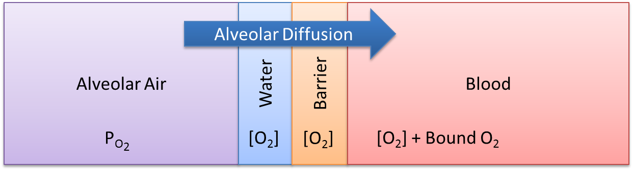
Gas Exchange - Alveoli Transfer
At the alveoli-pulmonary capillary interface, oxygen diffuses from the alveoli into the pulmonary capillaries, while carbon dioxide diffuses from the pulmonary capillaries into the alveoli. In reality, gas exchange at the alveoli is a multi-step process in space, where gases dissolve into liquid according to Henry's law and diffuse through liquid and across membranes according to Fick's law. In BioGears, alveolar gas exchange is driven by the partial pressure differential between the pulmonary capillaries and the alveoli in a one-step process, as shown in Figure 4. The partial pressures of each gas in the capillaries are calculated using Equation 3, while the partial pressures of each gas in the alveoli are calculated using Equation 4.
\[P_{P} = \frac{C}{d * C_{S}} \]
\[P_{P} = P * V_{f} \]
Where, Pp is the partial pressure, C is the concentration, d is the density, Cs is the solubility coefficient, P is the total pressure, and Vf is the volume fraction.
The diffusion rate is calculated using Equation 5 [134] .
\[\dot{D} = \frac{D_{co} * C_{D} * \Delta P_{P} * SA_{a}}{D_{d}} \]
Where Dco is the diffusing capacity of oxygen, CD is the relative diffusion coefficient, Pp is the partial pressure differential between the alveoli and the capillaries, SAa is the surface area of the alveoli, and Dd is the diffusion distance. The surface area of the alveoli for an individual patient is related to the standard alveoli surface area and the patient’s total lung capacity. This calculation is shown in Equation 6.
\[SA_{a} = \frac{TLC_{p}}{TLC_{s}} * SA_{as} \]
Where TLCp is the total lung capacity of the patient, as specified in the patient file (PatientData). TLCs is the standard healthy total lung capacity of 5.8 L [134] . The SAas is standard alveoli surface area of 70 square meters [134]. For more information about patient variability, please see the Patient Methodology report.
The mass diffused at each time step is calculated using Equation 7. This mass is either added or removed from the pulmonary capillaries and the corresponding volume is either added or removed from the alveoli.
\[D_{m} = \dot{D} * \Delta t * d \]
Instant Diffusion
Some substances are able to diffuse across biological membranes at a rate that ensures concentration equilibrium within one BioGears time step. The instant diffusion model is included in the BioGears Tissue system in order to simulate transport processes that fully evolve in a time period much smaller than the BioGears time step. All of the gases in BioGears are transported by instant diffusion, and in the current release, sodium is also transported by instant diffusion. Active pumping mechanism for ions are planned for a future release.
Simple Diffusion
Simple diffusion is an implementation of Fick's law in one dimension with a known constant distance. In this case, Fick's law can be described by Equation 8.
\[J_{X} = P_{x} * \left([X]_{v} - [X]_{t} \right) \]
Where Jx is the mass flux (mass per area-time) of substance X, *[X]v,t* is the concentration of substance X in compartment v (or t), and Px is a proportionality constant defining the permeability. The flux is multiplied by an area to obtain a rate of mass transfer. It is incredibly difficult to experimentally determine the capillary surface area for a given tissue, and it may be impossible to experimentally determine the total cellular membrane surface area. Additionally, lumped tissue models can be difficult to delineate. In BioGears, the capillary and cellular membrane surface areas are assumed to be proportional to the mass of a given organ or tissue group, such that the mass transfered in one time step (Dm) may be computed by Equation 9, where k is the empirically-determined constant relating the tissue mass (mt) to the surface area.
\[ D_{m} = k * m_{t} * J_{X} * \Delta t \]
In BioGears, simple diffusion is limited to substances with a molar mass under 1000 grams per mole.
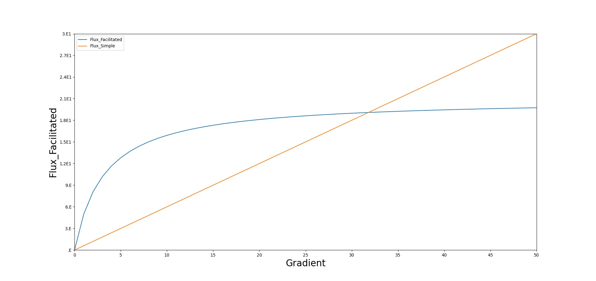
Facilitated Diffusion
Facilitated diffusion uses Michaelis-Menten kinetics to model the facilitated transport across a membrane. Note that this type of diffusion does not require energy and it is still a gradient-based transport mode. In contrast to simple diffusion, where substance flux can continue to increase with the concentration gradient, the flux is asymptotic in facilitated diffusion. The flux limit reflects a saturation of the membrane transporter mechanisms. However, at smaller concentration gradients, substance flux is higher in facilitated diffusion than with simple Fick's law diffusion. Figure 5 demonstrates the difference in flux between facilitated and simple diffusion. The mass flux given by Michaelis-Menten kinetics is computed using Equation  10;, where Jmax is the maximum flux and *Km is the Michaelis constant.
\[ J_{X} = \frac{\left([X]_{v} - [X]_{t} \right) * J_{max}}{K_{m} * \left([X]_{v} - [X]_{t} \right)} \]
In BioGears, glucose is the main substance moved by facillitated diffusion. Triacylglycerol and ketones are given flux values to increase their diffusion quantity as a way to model lipophilicity, though this is planned to be improved in a future release.
Active Transport
Active transport is currently utilized to shuttle the ions sodium, potassium, and chloride between the intracellular and extracellular tissue compartments. In doing so, concentration gradients characteristic of each ion are preserved (see Table 1). These ions were emphasized because they play diverse roles in facilitated transport of other compounds (i.e. sodium-glucose), cell signaling, and cell volume maintainance [134]. Volume regulation is currently implemented and discussed below, while the other functions remain areas of future work.
| Ion | Intracellular (mM) | Extracellular (mM) |
|---|---|---|
| Sodium | 15 | 145 |
| Potassium | 120 | 4.5 |
| Chloride | 4.5 | 102 |
Actively transported substances are unique in BioGears in that their movements are coupled. The motivation for this choice stems from the fact that ions are simultaneously subject to electromotive forces arising from the resting cell membrane potential (generally -60 to -90 mV, depending on the type of cell).
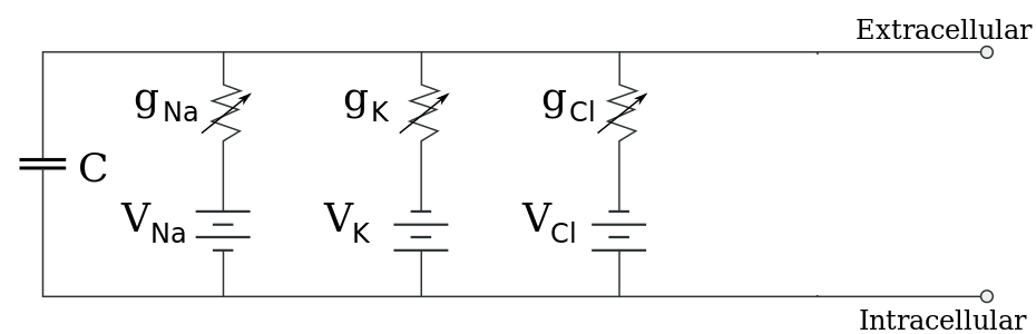
There are several approaches to modeling electrochemical flux, but the most useful for our purposes assumes that the cell membrane acts as a simple circuit (see Figure 6 below). The cell is assumed to possess a constant capacitance and selectively permeable ionic channels that serve as branches of current flow. Each channel has a characteristic conductance (inverse resistance) and a voltage equal to the Nernst potential of the ion in question.
The Nernst potential of Ion X, which accounts for the influence of both chemical and electrical driving forces, is given by
\[V_{x} = \frac{RT}{zF} * ln \left(\frac{C_{e}}{C_{i}} \right) \]
In Equation 11 [185], R is the Ideal Gas Constant (8.314 J/mol-K), T is body temperature in Kelvin, z is the charge of the Ion x, F is Faraday's Constant (96,485 C/mol), Ce is the extracellular concentration of Ion x, and Ci is the intracellular concentration of Ion x. If one assumes that each channel exhibits linear current-voltage (i.e. ohmic) behavior, the current across each pathway is
\[I_{x} = g_{x} \left(V_{m} - V_{x} \right) \]
where Vm is the total membrane potential [185]. By convention, a positive current is associated with movement directed from the intracellular to the extracellular space. The conductances (obtained from [410]) assume resting membrane permeability unassociated with action potential transmission. Equation 12 indicates that the larger the difference between an ion's Nernst potential and the membrane potential, the greater the current (flux) that ion will experience. Intuitively, when the Nernst potential is equal to the membrane potential, the ion will experience no net flux. These passive currents, if left unchecked, will disrupt the gradients shown in Table 1 and must be opposed by active transport. While cells employ a large number of transport mechanisms, we model only the Na-K-ATPase in the manner of [193] using parameters from [410].
\[P = P_{max}f_{NaK}\left( \frac{K_{e}}{K_{e}+k_{m,K}} \right) \left(\frac{1}{1 + \left(\frac{k_{m,Na}}{Na_{i}}\right)^{1.5}}\right)\]
\[f_{NaK} = \frac{1}{1 + 0.1245exp\left(\frac{-0.1V_{m}F}{RT}\right) + 0.2555exp\left(\frac{-V_{m}F}{RT}\right)\left(exp\left(\frac{Na_{e}}{67.3}\right)-1\right)}\]
The pump rate yielded by Equations 13-14 is in terms of the net number of cations moved during each pumping instance. The net movement of 1 cation is the result of pumping three sodium ions out of the cell and two potassium ions in to the cell. Thus, the transport rates of sodium and potassium (from an intracellular perspective) are 3P and -2P, respectively. The parameters km,K and km,Na are half-saturation values for the pump. The factor fNaK allows for the possibility of pump inhibition by extracellular Sodium. Pmax represents the maximum pumping rate and, as before, F is Faraday's constant and Vm is the membrane potential.
Combining Equations 12-14 yields the system of ionic fluxes in Equations 15-17. Chloride is assumed to undergo no active transport; rather, it is subject only to its electrochemical gradient. This assumption is consistent with a "Pump-Leak Model", in which chloride is allowed to leak across membrane channels to conserve both charge and osmotic pressures in the face of active potassium and sodium transport. It follows immediately that chloride concentrations must equilibrate in such a way to produce a Nernst potential identical to the membrane potential.
\[J_{Na} = -\left(\frac{I_{Na}}{F} + 3P \right) \]
\[J_{K} = -\left(\frac{I_{K}}{F} - 2P \right) \]
\[J_{Cl} = \frac{I_{Cl}}{F} \]
The negative signs in Equations 15 and 16 stem from the previously stated convention of positive current being directed outward. No negative sign is included in Equation 17 because Chloride has a negative charge and will thus travel in the opposite direction of a postive current. Division of the ionic currents by Faraday's constant renders them in a molar basis.
The presence of these ionic fluxes affects the resting membrane potential via the differential equation
\[-C\frac{dV_{m}}{dt} = \sum{}^{}I = g_{Na}*\left(V_{m} - V_{Na} \right) + g_{K}*\left(V_{m} - V_{K} \right) + g_{Cl}*\left(V_{m} - V_{Cl} \right) + FP\]
where C is the membrane capacitance. Equation 18, which implicitly guarantees conservation of charge, is frequently simplified in literature by making the assumption that the change in membrane potential occurs on a much faster time scale than the changes in ionic concentrations, allowing the approximation dVm/dt = 0 [13]. Equation 18 can then be arraged and solved for Vm
\[V_{m} = \frac{-FP + g_{Na}V_{Na} + g_{K}V_{K} + g_{Cl}V_{Cl}}{g_{Na} + g_{K} + g_{Cl}} \]
As mentioned above, ionic transport plays a prominent role in intracellular volume regulation. Water flows across the semi-permeable cell membrane in response to changes in osmotic pressure. We assume that the osmotic pressure on each side of the cell membrane is solely a function of Na, K, and Cl concentrations, with one caveat. A quick consultation of Table 1 reveals a drastic difference in the target total extracellular and intracellular molarities. These values would immediately lead to a significant osmotic pressure gradient. We follow the examples of [13] and [410] and lump the other anionic intracellular species into a single parameter, A-. We assume that the amount (in moles) of A- is sufficient to ensure isotonicity at our target concentrations. With this simplification, we can express the osmotic gradient as
\[\Delta \Pi = RT\left(Na_{i} + K_{i} + Cl_{i} + \frac{A^{-}}{W_{i}} - Na_{e}-K_{e}-Cl_{e}\right) \]
In Equation 20, Wi represents the current intracellular volume (W used to avoid confusion with membrane potential). The degree to which water is able to pass through the cell membrane is characterized by the membrane hydraulic conductivity, denoted Lp, which leads to the following equation for water flux:
\[J_{w} = L_{p}\Delta \Pi \]
There are biological limits to the amount of water that can be transported by this method, as cells can only tolerate mild fluctuations in volume (1-5%, depending on the cell [hernandez1998modeling]). However, we did not exceed these bounds during our testing due to the robustness of the Pump-Leak model. There is research to indicate that when cells approach intolerable volumes, rapid changes in ion concentrations are initiated to correct the osmotic gradient. This feature could be an interesting area of future modeling work, should it be required.
To summarize, at each time-step in BioGears, Equations 11-17, 19, and 20-21 are solved in order. The Nernst potentials of all ions are calculated, followed by the ionic channel currents, the pump current, and molar fluxes. The next membrane potential is calculated and stored for the subsequent time-step. The ionic concentrations are then used in Equations 20-21 to calculate water flux into the intracellular compartment. This flux is set on the flow source representing the cell membrane in Figure 3.
Metabolic Production and Consumption
In older versions of BioGears, metabolic production and consumption were calculated based on a respiratory quotient, using the O2 and CO2 values to back-calculate the amount of nutrients that must have been consumed. As of BioGears version 6.2, this functionality has been re-engineered to work in a more intuitive way. Now, the consumption and production in any given tissue is dependent on the nutrients available in that tissue and the desired metabolic rate.
The first step in the metabolic consumption and production method is to determine the amount of energy requested for the given timestep. This data is pulled from the Energy System, and it includes any exercise work. The next step is to portion out the energy demands to individual tissues. The brain requires a more or less constant portion of the body's total energy, about 20% [270], so this portion is set aside. The remaining portion of the energy requested is divided between the tissues of the body according to the amount of blood flow they receive. Though this assumption may not be 100% accurate, it follows that since the blood carries oxygen and nutrients to tissues, tissues that require more blood will also require more nutrients. This method allows us to leverage already validated blood flow rates and have the potential to add new organs without micromanaging consumption for every tissue.
The next step is to determine the stoichiometric relationships between nutrients during consumption and production. Metabolism is, at its most basic level, simply a collection of chemical reactions, a transferrance of energy from ingested food to ATP. But because BioGears doesn't model each and every substance and enzyme in the human body, the chemical reactions can't be completely characterized. However, the molar ratios between reactants and products can be used to ensure that the both the starting points and ending points of the reactions are captured. Table 1 below shows the chemical relationships used in BioGears' metabolic production and consumption.
| Chemical Relationship | Value | Notes |
|---|---|---|
| ATP produced per Glucose | 29.85 | [280] |
| CO2 produced per Glucose | 6 | |
| O2 consumed per Glucose | 6 | |
| ATP produced per Ketone | 24 | Assumed acetoacetate |
| CO2 produced per Ketone | 6 | |
| O2 consumed per Ketone | 6 | |
| ATP produced per Amino Acid | 13 | Assumed alanine |
| CO2 produced per Amino Acid | 1.5 | |
| O2 consumed per Amino Acid | 1.875 | |
| Urea produced per Amino Acid | .5 | |
| ATP produced per Triacylglycerol | 330 | Assumed tripalmitin [30] |
| CO2 produced per Triacylglycerol | 55 | [217] |
| O2 consumed per Triacylglycerol | 78 | |
| Aerobic ATP produced per Glycogen | ATP per Glucose + 1 (30.85) | [134] |
| Anaerobic ATP produced per Glycogen | 3 | |
| Anaerobic Lactate produced per Glycogen | 2 | |
| Anaerobic ATP produced per Glucose | 2 | |
| Anaerobic Lactate produced per Glucose | 2 |
One thing to be aware of is that not all of the energy contained in one mole of a given nutrient is converted to cellular work. For example, when burning glucose in a bomb calorimeter, 686 kcal/mol of energy is released [30]. In the body, however, glucose is converted to CO2, H2O, and energy by a series of reactions, none of which are as efficient as a bomb calorimeter. Thus, only a fraction of the energy in a given nutrient is used to perform cellular work; the rest is lost as heat. In order to calculate the efficiency of nutrient consumption, Equation 10 was used. These efficiency values were used for glucose, triacylglycerol, amino acids, and ketones according to [30], [380], and [187].
\[Efficiency=\frac{E_{ATP} *n_{ATP} }{E_{free} } \]
Where EATP is the energy released under cellular conditions per mole of ATP, nATP is the number of moles of ATP generated per mole of nutrient, and Efree is the free energy contained in one mole of nutrient.
In order to capture the appropriate nutrient responses of the body during exertion, nutrients are consumed in a certain order. Because the brain is so important to body function, its nutrient requirements are addressed first. It consumes glucose, and if none is available, it consumes ketones [134]. The BioGears brain cannot consume amino acids or triacylglycerol. Next, non-brain tissues are considered. Because the body has an obligatory protein requirement of 30 grams or more [134], amino acids are consumed next. Their rate of consumption is such that the body will always consume 30 grams a day, and this is increased under conditions where the hormone factor is low. Amino acid consumption produces urea as a byproduct, which is incremented in the liver, which, when combined with Hepatic gluconeogenesis, provides an abbreviated model of the Cori cycle. Next in line for consumption is triacylglycerol, the body's largest aerobic energy source. Consumption of triacylglycerol is rate-limited based on the hormone factor, with low hormone factors allowing for greater fat consumption. Next, aerobic glucose consumption via glycolysis and the citric acid cycle is considered. If the tissue in question is the muscle tissue, muscle glycogen can be used, first aerobically, then, in the absence of blood glucose, anaerobically. This ordering of consumption ensures that, under a resting state, the body tries to maintain its nutrient stores.
If at any time a tissue does not have the necessary oxygen or nutrient required to meet its energy demands, the deficit is logged as fatigue.
Protein/Fat Storage and Release
As the liver stores glucose in the form of glycogen to serve as an energy source in times of need, it also stores fat in the adipose tissue [134]. Protein doesn't have explicit storage in the same fashion, but it has been shown that about 1% of total body protein can be quickly broken down and metabolized during times of need [243]. This is not to be confused with muscle catabolism, which happens more slowly and after a longer period of time, and which is not modeled in BioGears. The functionality of fat and protein storage and release works very similarly to glycogenesis and glycogenolysis in the liver (see Hepatic Syetem). First, a local hormone factor is calculated, which is used to determine a rate of storage or release. These rates were determined empirically to give appropriate time courses of nutrient in the blood. Then, the substances are incremented accordingly.
Assumptions and Limitations
Proteins are large molecules that take up space. About 7% of plasma volume is due to proteins. Proteins also have a net negative charge. In reality, diffusion depends on the elctrochemical gradient, not just the chemical gradient. With the exception of the perfusion-limited diffusion model, the BioGears diffusion models do not account for the entire elecrochemical gradient or the volume of the protein in the plasma (i.e. no "plasma water").
The diffusional exchange of water between the capillaries and extravascular space amounts to as much as 80,000 liters per day. Convective capillary exchange is much less, on the order of 16 liters per day. The diffusional exchange of water is not modeled in BioGears.
The lipophilicity of molecules like triacylglycerol is not considered in BioGears' current diffusion method. If triacylglycerol was diffused only based on its considerable molar mass, it would hardly move at all in BioGears. To remedy this, some triacylglycerol is moved via facilitated diffusion by assigning it diffusion flux parameters.
The brain is currently the only tissue capable of metabolizing ketones, though in reality both myocardium and muscle can also consume ketones for energy. This limitation will be reexamined with upcoming changes to the modeling of starvation.
The muscle is considered as one lumped compartment in BioGears. For accurate modeling of consumption and production, especially in the case of isolated lactate production, discrete muscle compartments would give more accurate results.
Glucose diffusion is regulated by insulin level in many tissues, though this behavior is not modeled in BioGears.
Conditions
#Dehydration The dehydration condition is biogears is initialized as a fraction that corresponds to a decrease in patient weight from baseline. We assume that dehydration and extracellular fluid volume depletion are differing events with the latter corresponding to substance depletion in addition to fluid loss [203]. We are careful to not associate extracellular sodium with dehydration to allow for correct bedside assessment of the patient in regards to elevated solute concentrations in the fluid compartments of the body. The dehydration fraction determines how much weight the patient has lost as a result of fluid depletion, for example a 0.05 fraction corresponds to a 5 percent body weight decrease. We also support a patient event that informs the user when the patient has reached over 3 percent decrease in body weight. This is generally the threshold when active performance begins to decrease and obvious signs of fluid imbalance become prominent [48]. In addition BioGears will inform the user that the patient is thirsty at an increase of 3 percent plasma osmolarity.
This fraction is then used to reduce fluid volume levels across all fluid compartments within BioGears, including the vasculature [71]. We compute the fractional amount of fluid decrease in each compartment by first computing total water lost as a function of patient mass lost:
V = {M_P}( {{{{M_{frac}}}}{ }} ). ]
Here MP is the baseline patient weight (generally initialized in the patient file), Mfrac is the fractional weight lost due to dehydration, set by the condition, and ** is the standard density of water at internal body temperatures. We then scale to get a fractional fluid lost by dividing through by total body water. This value is then multiplied by the extracellular, intracellular, and vascular fluid compartments to get total fluid lost in each.
Validated data is mostly qualitative for a 5 percent patient weight decrease from baseline due to fluid loss. The condition does well for total body water reductions, patient weight decrease, and plasma osmolarity increases, table 4. This allows for a clinician to properly diagnose the condition in a training scenario.
For significant dehydration (> 5 percent) it is known that performance at submaximal exercise and in variable environmental conditions increases heart rate and decrease stroke volume [48]. These cardiovascular deficiencies have not been tested for our virtual patient but could be an interesting lead into future work. Due to the strenuous and variable nature of testing dehydrated patients during exercise, at altitude, and in varying hot/cold environments, having a computational tool and validated model to determine performance to the soldier or athlete would be useful.
| Condition | Notes | Sampled Scenario Time (s) | Body Weight | Aorta Sodium Concentration | Blood Volume |
|---|---|---|---|---|---|
| 5% body weight dehydration condition applied | Dehydration condition is applied as a reduction of patient weight from baseline | 60 | Decrease [307] | Increase [307] | Decrease [307] |
Actions
At this time, there are no insults or interventions associated with the Tissue system. Other system actions can affect the diffusion properties or other transports by modifying the diffusion surface area. An example of this is found in the Respiratory Methodology for lobar pneumonia. As the alveoli fill with fluid, they are unable to participate in gas exchange. This reduces the alveoli surface area, which leads to a reduction of available oxygen in the CardiovascularSystem and the EnergySystem.
Events
- Dehydration: Set when fluid loss exceeds 3% of body mass [390]
- Thirst: Set when plasma osmolarity increases 2% [48]
Results and Conclusions
Verification
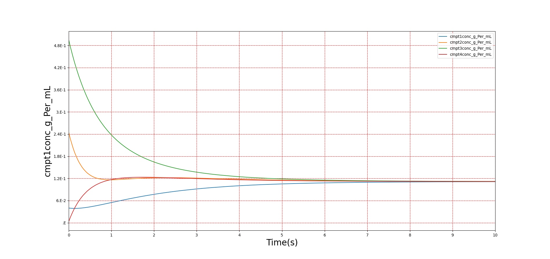
Verification of the diffusion methods is achieved through several units tests. One of the simple diffusion unit tests was used to generate data for Figure 7. The figure shows the time-evolution of the concentrations of four different compartments. Table 3 shows the initial conditions. Note that the units are arbitrary, thus not shown. The red, blue, and green compartment all share a boundary with the yellow compartment, but not with each other.
| Compartment | Volume | Mass | Concentration |
|---|---|---|---|
| Red | 50.0 | 2.0 | 0.04 |
| Blue | 10.0 | 2.5 | 0.20 |
| Green | 20.0 | 10 | 0.50 |
| Yellow | 50.0 | 0.0 | 0.00 |
Validation - Resting Physiologic State
The tissue system volumes are validated using data from [374].
| Tissue | Expected Value | Engine Value | Percent Error | Notes |
|---|---|---|---|---|
| ExtracellularFluidVolume(mL) | 8819.820000[374] | 9441.110815 | 6.804591% | Excluding intravascular fluid |
| ExtravascularFluidVolume(mL) | 34138.680000[374] | 34411.508082 | 0.795995% | |
| IntracellularFluidPH | [6.000000,7.400000][134] | 7.000000 | Within Bounds | |
| IntracellularFluidVolume(mL) | 25320.000000[374] | 24970.395267 | 1.390344% | Excluding intravascular fluid |
| LiverGlycogen(g) | [0.000000,120.000000][30] | 117.000000 | Within Bounds | |
| OxygenConsumptionRate(mL/min) | 250.000000guyton2006medical | 241.581847 | 3.424924% | |
| RespiratoryExchangeRatio | 0.850000[128] | 0.878500 | 3.297666% |
| TissueCompartments | Expected Value | Engine Value | Percent Error | Notes |
|---|---|---|---|---|
| BoneTissueExtracellular-Volume(mL) | 808.000000[149] | 873.591901 | 7.801168% | |
| BoneTissueIntracellular-Volume(mL) | 2795.680000[149] | 2727.869355 | 2.455329% | |
| BrainTissueExtracellular-Volume(mL) | 234.900000[149] | 249.255291 | 5.930036% | |
| BrainTissueIntracellular-Volume(mL) | 899.000000[149] | 883.961673 | 1.686893% | |
| FatTissueExtracellular-Volume(mL) | 2127.600000[149] | 2391.967672 | 11.698804% | |
| FatTissueIntracellular-Volume(mL) | 267.920000[149] | 283.115981 | 5.515422% | |
| GutTissueExtracellular-Volume(mL) | 287.640000[149] | 297.743543 | 3.451939% | |
| GutTissueIntracellular-Volume(mL) | 484.500000[149] | 474.348775 | 2.117378% | |
| LeftKidneyTissueExtracellular-Volume(mL) | 42.315000[149] | 44.000000 | 3.904304% | |
| LeftKidneyTissueIntracellular-Volume(mL) | 74.865000[149] | 73.159640 | 2.304157% | |
| LeftLungTissueExtracellular-Volume(mL) | 84.000000[149] | 86.000000 | 2.352941% | |
| LeftLungTissueIntracellular-Volume(mL) | 111.500000[149] | 109.168805 | 2.112845% | |
| LiverTissueExtracellular-Volume(mL) | 289.800000[149] | 309.152641 | 6.462161% | |
| LiverTissueIntracellular-Volume(mL) | 1031.400000[149] | 1011.565739 | 1.941713% | |
| MuscleTissueExtracellular-Volume(mL) | 3422.000000[149] | 3633.950508 | 6.007710% | |
| MuscleTissueIntracellular-Volume(mL) | 18270.000000[149] | 18056.200967 | 1.177106% | |
| MyocardiumTissueExtracellular-Volume(mL) | 105.600000[149] | 108.618230 | 2.817902% | |
| MyocardiumTissueIntracellular-Volume(mL) | 150.480000[149] | 147.401266 | 2.067088% | |
| RightKidneyTissueExtracellular-Volume(mL) | 42.315000[149] | 44.000000 | 3.904304% | |
| RightKidneyTissueIntracellular-Volume(mL) | 74.865000[149] | 73.159640 | 2.304157% | |
| RightLungTissueExtracellular-Volume(mL) | 84.000000[149] | 86.000000 | 2.352941% | |
| RightLungTissueIntracellular-Volume(mL) | 111.500000[149] | 109.169472 | 2.112234% | |
| SkinTissueExtracellular-Volume(mL) | 1260.600000[149] | 1284.723713 | 1.895532% | |
| SkinTissueIntracellular-Volume(mL) | 960.300000[149] | 935.724046 | 2.592367% | |
| SpleenTissueExtracellular-Volume(mL) | 31.050000[149] | 32.732211 | 5.274860% | |
| SpleenTissueIntracellular-Volume(mL) | 86.850000[149] | 85.138810 | 1.989885% |
More validation of this system can be found in the system outputs of all other systems, e.g., the oxygen and carbon dioxide saturation, the blood pH, and the bicarbonate concentration values are found in the Blood Chemistry Methodology and the alveoli oxygen and carbon dioxide partial pressures are found in the Respiratory Methodology.
Validation - Actions and Conditions
There are currently no validated actions or conditions associated with the Tissue system. However, there will be condition validation after improvements are made to the dehydration and starvation condition models.
Future Work
Coming Soon
- Albumin transport model to affect blood albumin concentration based on hepatic production and to model changes in plasma colloid oncotic pressure.
Recommended Improvements
- Permeability-limited diffusion model
- Endogenous carbon monoxide production
- Muscle catabolism
- Insulin effects on glucose diffusion
Appendices
Data Model Implementation
Tissue
Compartments
- Bone
- BoneExtracellular
- BoneIntracellular
- Brain
- BrainExtracellular
- BrainIntracellular
- Fat
- FatExtracellular
- FatIntracellular
- Gut
- GutExtracellular
- GutIntracellular
- LeftKidney
- LeftKidneyExtracellular
- LeftKidneyIntracellular
- LeftLung
- LeftLungExtracellular
- LeftLungIntracellular
- Liver
- LiverExtracellular
- LiverIntracellular
- Muscle
- MuscleExtracellular
- MuscleIntracellular
- Myocardium
- MyocardiumExtracellular
- MyocardiumIntracellular
- RightKidney
- RightKidneyExtracellular
- RightKidneyIntracellular
- RightLung
- RightLungExtracellular
- RightLungIntracellular
- Skin
- SkinExtracellular
- SkinIntracellular
- Spleen
- SpleenExtracellular
- SpleenIntracellular
- Lymph